
Figure 6.1: Two-dimensional velocity field observations
In this chapter, we will explain the GPU implementation of Curl Noise, which is a pseudo-fluid algorithm.
The sample in this chapter is "Curl Noise" from
https://github.com/IndieVisualLab/UnityGraphicsProgramming2
.
Curl Noise is a pseudo-fluid noise algorithm announced in 2007 by Professor Robert Bridson of the University of British Columbia, who is also known as a developer of fluid algorithms such as the FLIP method.
In the previous work "Unity Graphics Programming vol.1", I explained the fluid simulation using the Navier-Stokes equation, but Curl Noise is a pseudo but light load compared to those fluid simulations. It is possible to express fluid.
In particular, with the recent advances in display and projector technology, there is an increasing need for real-time rendering at high resolutions such as 4K and 8K, so low-load algorithms such as Curl Noise can express fluids in high resolution and low resolution. It is a useful option for expressing with machine specifications.
In fluid simulation, the first thing you need is a vector field called the "velocity field". First, let's imagine what a velocity field is like.
Below is an image of the velocity field in two dimensions. You can see that the vector is defined at each point on the plane.
Figure 6.1: Two-dimensional velocity field observations
As shown in the above figure, the state in which each vector is individually defined in each differential interval on the plane is called a vector field, and the one in which each vector is a velocity is called a velocity field.
Even if these are three-dimensional, it is easy to understand if you can imagine that the vector is defined in each differential block in the cube.
Now let's see how Curl Noise derives this velocity field.
The interesting thing about Curl Noise is that it uses gradient noise such as Perlin Noise and Simplex Noise, which was explained in the previous chapter "Introduction to Procedural Noise", as a potential field, and derives the velocity field of the fluid from it.
In this chapter, we will use 3D Simplex Noise as a potential field.
Below, I would like to first unravel the algorithm from the Curl Noise formula.
\overrightarrow{u} = \nabla \times \psi
The above is the Curl Noise algorithm.
The left side \ overright arrow {u} is the derived velocity vector, the right side \ nabla is the vector differential operator (read as nabla, which acts as an operator of partial differential), and \ psi is the potential field. (3D Simplex Noise in this chapter)
Curl Noise can be expressed as the cross product of the two terms on the right side.
In other words, Curl Noise is Simple x Noise and partial differential of each vector element \ left (\ dfrac {\ partial} {\ partial x} _, \ dfrac {\ partial} {\ partial y} _, \ dfrac {\ partial} { It is the outer product of \ partial z} \ right) , and for those who have learned vector analysis in the past, you can see that it is the shape of rotA itself.
Now let's calculate the outer product of 3D Simplex Noise and partial derivative
\overrightarrow{u} = \left( \dfrac {\partial \psi _3} {\partial y} - \dfrac {\partial \psi _2} {\partial z}_, \dfrac {\partial \psi _1} {\partial z} - \dfrac {\partial \psi _3} {\partial x}_, \dfrac {\partial \psi _2} {\partial x} - \dfrac {\partial \psi _1} {\partial y} \right)
In general, the outer product is characterized by the fact that the two vectors are oriented vertically to each other and their length is the same as the area of the surface stretched by both vectors, but rotA (rotation) in vector analysis. ) Is a simple way to grasp the image of the cross product operation from the above formula, saying, "Look up the vector of the potential field in each twisted partial differential element direction, and pull the terms together, so rotation occurs." It may be easier to grasp the image if you capture it in.
The implementation itself is very simple, looking up the vector from each point of \ psi above , that is, 3D SimplexNoise, while slightly shifting the lookup point in the direction of each element of partial differentiation, and performing the outer product operation like the above formula. Just do.
If you have read the fluid simulation chapter of the previous work "Unity Graphics Programming vol.1", you may be wondering what the law of conservation of mass is.
The law of conservation of mass is that at each point in the velocity field, the inflow and outflow are always balanced, the inflow is outflowed, the outflow is inflowed, and finally the divergence is zero (divergence free). It was a rule.
\nabla \cdot \overrightarrow{u} = 0
This is also mentioned in the paper, but since the gradient noise itself changes gently in the first place (when imagining with a two-dimensional gradation, if the pixel on the left side is thin, the pixel on the right side is dark (As you can see), divergence-free was guaranteed at the time of the potential field. Considering the characteristics of Perlin noise, it is quite natural.
Now, let's implement the CurlNoise function on the GPU with Compute shader or Shader based on the formula.
#define EPSILON 1e-3

float3 CurlNoise (float3 coord)
{
    float3 dx = float3(EPSILON, 0.0, 0.0);
    float3 dy = float3 (0.0, EPSILON, 0.0);
    float3 dz = float3(0.0, 0.0, EPSILON);

    float3 dpdx0 = snoise(coord - dx);
    float3 dpdx1 = snoise(coord + dx);
    float3 dpdy0 = snoise(coord - dy);
    float3 dpdy1 = snoise(coord + dy);
    float3 dpdz0 = snoise(coord - dz);
    float3 dpdz1 = snoise(coord + dz);

    float x = dpdy1.z - dpdy0.z + dpdz1.y - dpdz0.y;
    float y = dpdz1.x - dpdz0.x + dpdx1.z - dpdx0.z;
    float z = dpdx1.y - dpdx0.y + dpdy1.x - dpdy0.x;

    return float3(x, y, z) / EPSILON * 2.0;
}
As mentioned above, this algorithm can be reduced to a simple four arithmetic operation, so the implementation itself is very easy, and it can be implemented with just this number of lines.
Below is a sample of Curl Noise implemented in the compute shader this time. It is possible to advect particles of particles, add a rising vector to make it look like a flame, and bring out various expressions depending on the idea.
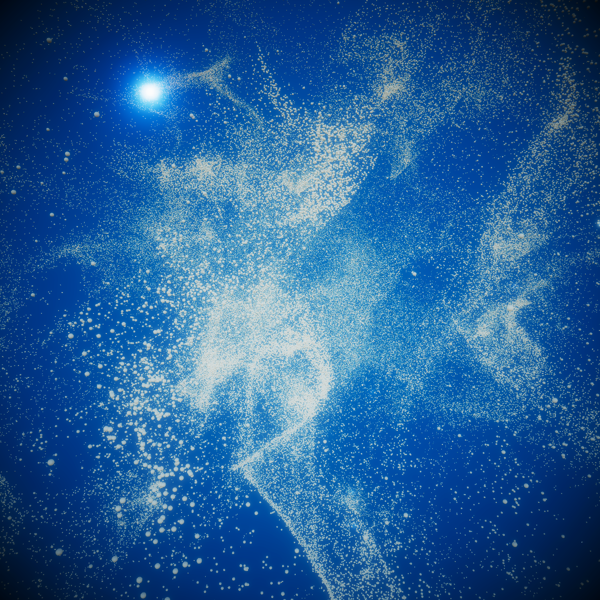
Figure 6.2:
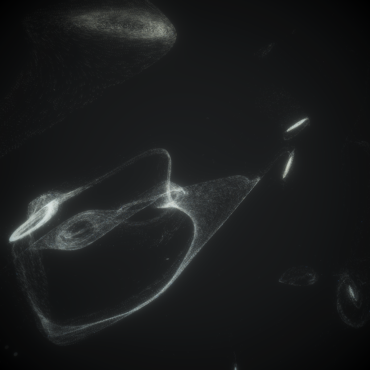
Figure 6.3:
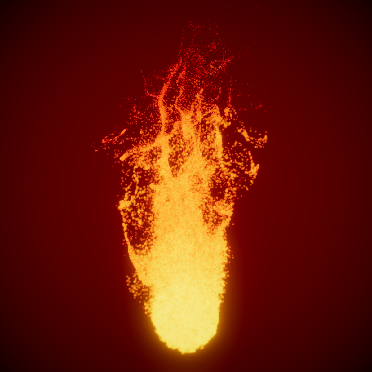
Figure 6.4:
In this chapter, we explained the implementation of pseudo-fluid by Curl Noise.
Since it is possible to reproduce a 3D pseudo-fluid with a small load and implementation, it is an algorithm that works especially useful for real-time rendering at high resolution.
In summary, I would like to conclude this chapter with the utmost thanks to Professor Robert Bridson, who is still discovering various techniques, including the Curl Noise algorithm.
I think there were some points that could not be explained and some parts were difficult to understand, but I hope that readers will enjoy graphics programming as well.